How to Make Graph Paper in Excel

If you wish to print graph paper from Excel, adjust cell width and height and change print margins.

Adjust the Size of All Cells

The first step is to change the dimension of cells in the worksheet. To adjust the height of all cells:

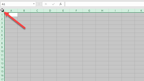
1. Select all cells in the worksheet by clicking the arrow in the upper-right corner (or pressing CTRL + A).

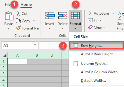
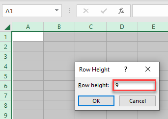
1. In the pop-up window, enter a Row height of 9 and click OK.
   Now the height of all cells in the current worksheet is set to 9.

1. Next, adjust the width of all cells. Select all cells in the worksheet, and then in the Ribbon, go to Home > Format and choose Column Width…

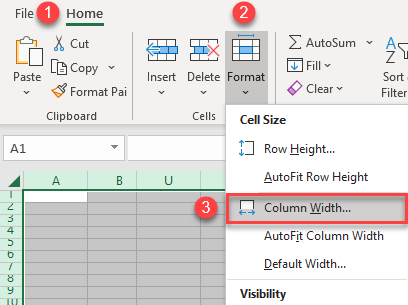
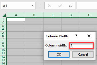
As a result, all cells have the same width and height. To proceed to print, set up the page layout.

Page Setup: Margins and Gridlines

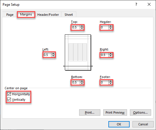
First, change the margins of the document.

1. In the Ribbon, go to Page Layout > Margins and choose Custom Margins…

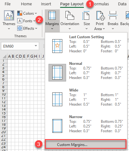adjust custom margins 1" width="412" height="482" />

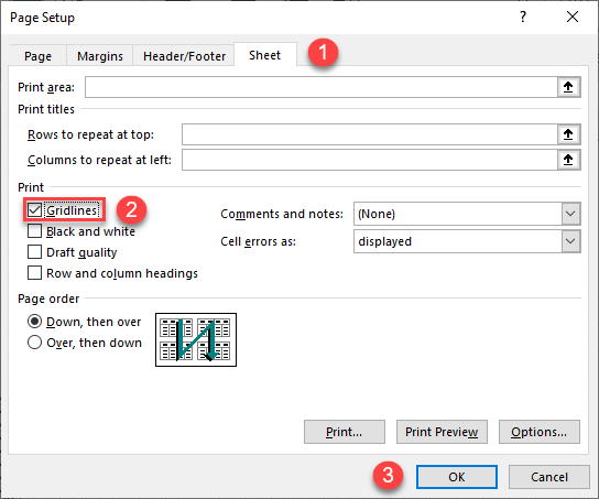
1. 1. Then go to the Sheet tab, and under Print, check Gridlines. Now we’ve enabled the printing of gridlines, which is necessary for printing graph paper.

   

   Print Graph Paper

   After making the changes above, you can print the document.

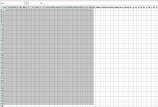
   1. Select the page range in the worksheet.

   

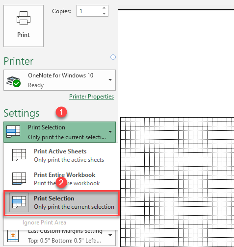
   1. Under Settings, in the first option, instead of default Print Active Sheets, choose Print Selection. This prints just the selection from the worksheet.

   

   The result is a sheet of graph paper available for printing in Excel, as you can see in Print Preview.